cell2clone - identifying lymphocyte clonal expansions from a single-cell dataset
[1]:
import scanpy as sc
import pandas as pd
import numpy as np
import matplotlib.pyplot as plt
import seaborn as sns

import cell2clone as c2c

%config InlineBackend.figure_format = "retina"

import warnings
warnings.filterwarnings("ignore")
In this notebook we demonstrate the use of cell2clone to estimate clonality of cell type compartments across samples, and subsequently to assign single cells into clones in highly clonal samples. Taking advantage of mutually exclusive expression of immunoglobulin light chains (IGKC/IGLC) in single B cells, and T cell receptor constant chains (TRBC1/TRBC2) in single T cells, cell2clone classifies each B or T cell into kappa/lambda or TRBC1/TRBC2 classes to infer clonal restriction within phenotypically defined cell populations. Non-clonal cells, such as naïve B or T cells show constant proportions of the two classes across samples, whereas cell types containing clonal expansions exhibit skewing of the fraction to either class in samples harbouring clonal expansions.
[2]:
# Load data (https://covid19.cog.sanger.ac.uk/submissions/release1/BCR_Moderate.h5ad, from https://www.covid19cellatlas.org/index.patient.html)
adata = sc.read_h5ad("data/BCR_Moderate.h5ad")
We load a dataset of B cells from COVID-19 patients (Stephenson et al. Nature Medicine 2021) with paired transcriptome and BCR sequencing data. Cell2clone is specifically intended for datasets without VDJ data. Here we use BCR sequencing information to validate cell2clone inferences.
[3]:
adata
[3]:
AnnData object with n_obs × n_vars = 11613 × 31279
    obs: 'sample_id', 'n_genes', 'n_genes_by_counts', 'total_counts', 'total_counts_mt', 'pct_counts_mt', 'leiden', 'initial_clustering', 'Resample', 'Collection_Day', 'patient_id', 'Sex', 'Age', 'Ethnicity', 'Swab_result', 'Status', 'Smoker', 'Status_on_day_collection', 'Status_on_day_collection_summary', 'Status_3_days_post_collection', 'Status_7_days_post_collection', 'Days_from_onset', 'Site', 'time_after_LPS', 'Worst_Clinical_Status', 'Outcome', 'filter_rna', 'has_bcr', 'filter_bcr_quality', 'filter_bcr_heavy', 'filter_bcr_light', 'bcr_QC_pass', 'filter_bcr', 'initial_clustering_B', 'leiden_B', 'leiden_B2', 'celltype_B', 'celltype_B_v2', 'clone_id', 'clone_id_by_size', 'isotype', 'lightchain', 'status', 'vdj_status', 'productive', 'umi_counts_heavy', 'umi_counts_light', 'v_call_heavy', 'v_call_light', 'j_call_heavy', 'j_call_light', 'c_call_heavy', 'c_call_light', 'clone_centrality', 'clone_degree', 'clone_id_size', 'mu_freq_heavy', 'mu_freq_light', 'clone_id_size_max_3', 'clone_network_cluster_size_gini', 'clone_network_vertex_size_gini', 'clone_size_gini', 'clone_centrality_gini', 'junction_heavy', 'junction_light', 'junction_aa_heavy', 'junction_aa_light'
    var: 'feature_types', 'highly_variable', 'means', 'dispersions', 'dispersions_norm'
    uns: 'Site_colors', 'Status_on_day_collection_summary_colors', 'bcr_QC_pass_colors', 'celltype_B_colors', 'celltype_B_v2_colors', 'filter_bcr_colors', 'hvg', 'initial_clustering_colors', 'isotype_colors', 'leiden', 'leiden_B_colors', 'leiden_colors', 'neighbors', 'pca', 'rank_genes_groups', 'rna_neighbors', 'umap'
    obsm: 'X_bcr', 'X_pca', 'X_pca_harmony', 'X_umap'
    obsp: 'bcr_connectivities', 'bcr_distances', 'connectivities', 'distances', 'rna_connectivities', 'rna_distances'
[4]:
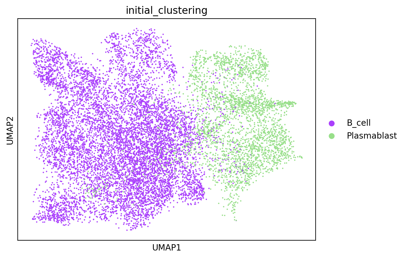
# Visualise broad cell types
sc.pl.umap(adata, color="initial_clustering")
[5]:
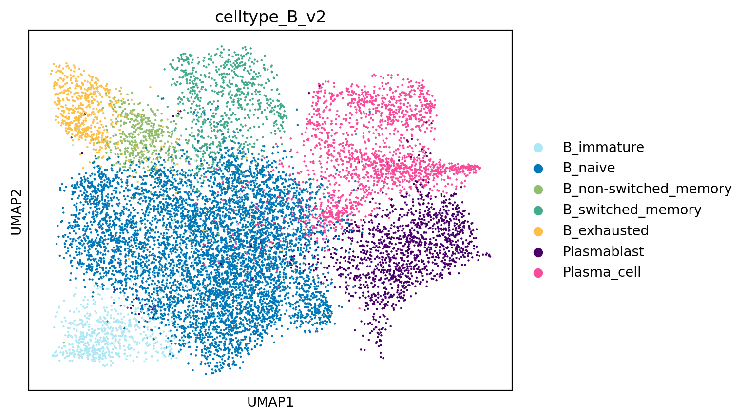
# Visualise fine-grained cell types
sc.pl.umap(adata, color="celltype_B_v2")
[6]:
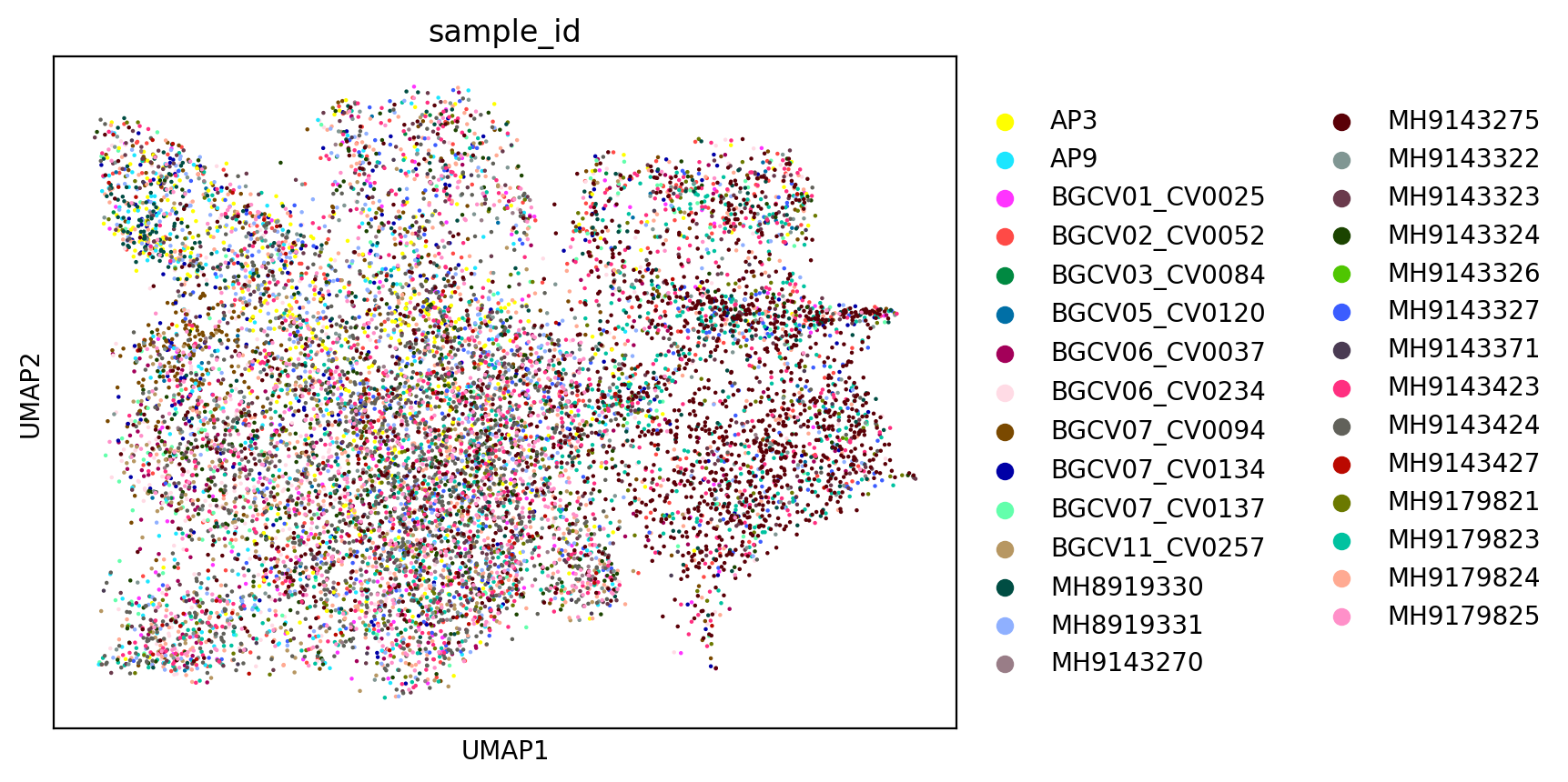
# Visualise sample IDs
sc.pl.umap(adata, color="sample_id")
[7]:
# Subset to B cells for simplicity
adata = adata[adata.obs["initial_clustering"].isin(["B_cell"])]
Classifying single cells based on light chain or constant chain usage
[8]:
# Define metadata columns to use
celltype = "celltype_B_v2"
sample = "sample_id"
We define each B cell as a kappa type if the expression of kappa gene is higher than a gene set of lambda genes, and as lambda type if the expression of the lambda gene set is higher thankappa gene expression. For T cells, we do the same using β-chain constant region genes TRBC1 and TRBC2. Cells in which neither gene or gene set is detected are classified as ambiguous.
[9]:
# Classify light chain class (B cells) or constant chain class (T cells) for each cell
c2c.classify_lightchain_or_trbc(
    adata,
    mode="B" # mode="T" if working with T cells
)
[10]:
adata
[10]:
AnnData object with n_obs × n_vars = 8604 × 31279
    obs: 'sample_id', 'n_genes', 'n_genes_by_counts', 'total_counts', 'total_counts_mt', 'pct_counts_mt', 'leiden', 'initial_clustering', 'Resample', 'Collection_Day', 'patient_id', 'Sex', 'Age', 'Ethnicity', 'Swab_result', 'Status', 'Smoker', 'Status_on_day_collection', 'Status_on_day_collection_summary', 'Status_3_days_post_collection', 'Status_7_days_post_collection', 'Days_from_onset', 'Site', 'time_after_LPS', 'Worst_Clinical_Status', 'Outcome', 'filter_rna', 'has_bcr', 'filter_bcr_quality', 'filter_bcr_heavy', 'filter_bcr_light', 'bcr_QC_pass', 'filter_bcr', 'initial_clustering_B', 'leiden_B', 'leiden_B2', 'celltype_B', 'celltype_B_v2', 'clone_id', 'clone_id_by_size', 'isotype', 'lightchain', 'status', 'vdj_status', 'productive', 'umi_counts_heavy', 'umi_counts_light', 'v_call_heavy', 'v_call_light', 'j_call_heavy', 'j_call_light', 'c_call_heavy', 'c_call_light', 'clone_centrality', 'clone_degree', 'clone_id_size', 'mu_freq_heavy', 'mu_freq_light', 'clone_id_size_max_3', 'clone_network_cluster_size_gini', 'clone_network_vertex_size_gini', 'clone_size_gini', 'clone_centrality_gini', 'junction_heavy', 'junction_light', 'junction_aa_heavy', 'junction_aa_light', 'kappa_sum', 'lambda_sum', 'KL_class', 'KL_log_ratio'
    var: 'feature_types', 'highly_variable', 'means', 'dispersions', 'dispersions_norm'
    uns: 'Site_colors', 'Status_on_day_collection_summary_colors', 'bcr_QC_pass_colors', 'celltype_B_colors', 'celltype_B_v2_colors', 'filter_bcr_colors', 'hvg', 'initial_clustering_colors', 'isotype_colors', 'leiden', 'leiden_B_colors', 'leiden_colors', 'neighbors', 'pca', 'rank_genes_groups', 'rna_neighbors', 'umap', 'sample_id_colors'
    obsm: 'X_bcr', 'X_pca', 'X_pca_harmony', 'X_umap'
    obsp: 'bcr_connectivities', 'bcr_distances', 'connectivities', 'distances', 'rna_connectivities', 'rna_distances'
[11]:
# Check added columns
adata.obs[[celltype, "kappa_sum", "lambda_sum", "KL_class", "KL_log_ratio"]] # for T cells "TRBC1_sum", "TRBC2_sum", "TRBC_class", "TRBC_log_ratio"]
[11]:
| celltype_B_v2 | kappa_sum | lambda_sum | KL_class | KL_log_ratio | |
|---|---|---|---|---|---|
| BGCV01_AACCATGTCATTCACT-1 | B_naive | 1.192134 | 0.000000 | kappa | 13.991257 |
| BGCV01_AACCGCGAGCGTGAAC-1 | B_naive | 0.000000 | 0.000000 | ambiguous | 0.000000 |
| BGCV01_AACTCAGGTGGCGAAT-1 | B_naive | 1.965800 | 4.370118 | lambda | -0.798891 |
| BGCV01_AACTCCCCAGTGGAGT-1 | B_naive | 0.000000 | 1.927203 | lambda | -14.471581 |
| BGCV01_ACATGGTAGCTCTCGG-1 | B_immature | 0.000000 | 4.017279 | lambda | -15.206116 |
| ... | ... | ... | ... | ... | ... |
| TTTACTGTCAAGGCTT-MH9179825 | B_naive | 1.384348 | 0.000000 | kappa | 14.140740 |
| TTTATGCCACATTTCT-MH9179825 | B_naive | 0.000000 | 2.449453 | lambda | -14.711376 |
| TTTCCTCAGACTAAGT-MH9179825 | B_naive | 1.950898 | 0.000000 | kappa | 14.483801 |
| TTTGGTTCAGGAATCG-MH9179825 | B_naive | 2.209406 | 0.000000 | kappa | 14.608234 |
| TTTGTCACAGAGTGTG-MH9179825 | B_naive | 0.000000 | 0.000000 | ambiguous | 0.000000 |
8604 rows × 5 columns
We see that most cells have been classified to either kappa or lambda light chain, while a minority remain ambiguous as neither gene is detected, likely due to dropouts.
Identifying clonal expansions across cell types and samples
We compute median-centered log2 ratio of kappa and lambda cells for each cell type in each sample. This metric will be highly positive or negative in cell types and samples harbouring large clonal expansions, and close to 0 in fully polyclonal cell populations. We additionally derive a directionless clonality metric as the absolute value of the log2 ratio and clone size score to quantify the deviation of the largest clone fraction of each cell type from the expected value in a fully polyclonal cell population. A score of 0 indicates that the observed clone fraction equals the expected value (i.e. fully polyclonal population), whereas a score of 1 corresponds to the largest possible deviation (i.e. fully monoclonal population).
We set the minimum number of cells required for clonality estimation relatively high (40 cells) to increase confidence. This also makes sense as we are looking for clonal expansions.
[12]:
# Estimate clonality for each cell type for each donor
df_class = c2c.compute_sample_celltype_clonality(
    adata,
    sample_col=sample,
    celltype_col=celltype,
    class_col="KL_class",
    state_labels=("kappa", "lambda"),
    clone_score_method="global",
    min_cells=40,
)
[13]:
columns_to_list = [sample, celltype, "kappa", "lambda", "frac_kappa", "KL_class_log2_ratio_scaled", "clonality", "clone_size_score"]
[14]:
df_class.sort_values("clone_size_score", ascending=False)[columns_to_list].head(60)
[14]:
| sample_id | celltype_B_v2 | kappa | lambda | frac_kappa | KL_class_log2_ratio_scaled | clonality | clone_size_score | |
|---|---|---|---|---|---|---|---|---|
| 78 | MH8919330 | B_exhausted | 50 | 2 | 0.961538 | 4.335733 | 4.335733 | 0.738166 |
| 51 | BGCV07_CV0094 | B_naive | 207 | 12 | 0.945205 | 3.800402 | 3.800402 | 0.708641 |
| 4 | AP3 | B_exhausted | 40 | 10 | 0.800000 | 1.691878 | 1.691878 | 0.446154 |
| 146 | MH9143424 | B_switched_memory | 32 | 10 | 0.761905 | 1.369950 | 1.369950 | 0.377289 |
| 68 | BGCV11_CV0257 | B_naive | 154 | 54 | 0.740385 | 1.203777 | 1.203777 | 0.338388 |
| 143 | MH9143424 | B_immature | 34 | 57 | 0.373626 | -1.053549 | 1.053549 | 0.324598 |
| 58 | BGCV07_CV0134 | B_naive | 68 | 25 | 0.731183 | 1.135484 | 1.135484 | 0.321754 |
| 63 | BGCV07_CV0137 | B_naive | 47 | 20 | 0.701493 | 0.924538 | 0.924538 | 0.268083 |
| 1 | AP3 | B_naive | 107 | 47 | 0.694805 | 0.878756 | 0.878756 | 0.255994 |
| 21 | BGCV02_CV0052 | B_naive | 67 | 31 | 0.683673 | 0.803771 | 0.803771 | 0.235871 |
| 136 | MH9143423 | B_immature | 17 | 23 | 0.425000 | -0.744221 | 0.744221 | 0.231731 |
| 102 | MH9143322 | B_naive | 44 | 58 | 0.431373 | -0.706672 | 0.706672 | 0.220211 |
| 177 | MH9179825 | B_naive | 190 | 98 | 0.659722 | 0.647023 | 0.647023 | 0.192575 |
| 109 | MH9143323 | B_naive | 71 | 86 | 0.452229 | -0.584640 | 0.584640 | 0.182509 |
| 8 | AP9 | B_naive | 27 | 32 | 0.457627 | -0.553235 | 0.553235 | 0.172751 |
| 38 | BGCV06_CV0037 | B_naive | 83 | 45 | 0.648438 | 0.575064 | 0.575064 | 0.172175 |
| 116 | MH9143324 | B_naive | 100 | 55 | 0.645161 | 0.554374 | 0.554374 | 0.166253 |
| 97 | MH9143275 | B_switched_memory | 24 | 27 | 0.470588 | -0.478047 | 0.478047 | 0.149321 |
| 82 | MH8919331 | B_naive | 55 | 61 | 0.474138 | -0.457500 | 0.457500 | 0.142905 |
| 137 | MH9143423 | B_naive | 77 | 85 | 0.475309 | -0.450727 | 0.450727 | 0.140788 |
| 163 | MH9179823 | B_naive | 71 | 74 | 0.489655 | -0.367829 | 0.367829 | 0.114854 |
| 130 | MH9143371 | B_naive | 37 | 38 | 0.493333 | -0.346596 | 0.346596 | 0.108205 |
| 123 | MH9143327 | B_naive | 44 | 44 | 0.500000 | -0.308122 | 0.308122 | 0.096154 |
| 144 | MH9143424 | B_naive | 299 | 285 | 0.511986 | -0.238939 | 0.238939 | 0.074486 |
| 95 | MH9143275 | B_naive | 135 | 127 | 0.515267 | -0.219991 | 0.219991 | 0.068555 |
| 44 | BGCV06_CV0234 | B_naive | 87 | 61 | 0.587838 | 0.204084 | 0.204084 | 0.062630 |
| 139 | MH9143423 | B_switched_memory | 23 | 21 | 0.522727 | -0.176878 | 0.176878 | 0.055070 |
| 157 | MH9179821 | B_naive | 69 | 62 | 0.526718 | -0.153794 | 0.153794 | 0.047857 |
| 15 | BGCV01_CV0025 | B_naive | 39 | 29 | 0.573529 | 0.119299 | 0.119299 | 0.036765 |
| 170 | MH9179824 | B_naive | 129 | 113 | 0.533058 | -0.117074 | 0.117074 | 0.036395 |
| 89 | MH9143270 | B_naive | 43 | 33 | 0.565789 | 0.073748 | 0.073748 | 0.022773 |
| 172 | MH9179824 | B_switched_memory | 32 | 25 | 0.561404 | 0.048022 | 0.048022 | 0.014845 |
| 75 | MH8919330 | B_naive | 26 | 21 | 0.553191 | 0.000000 | 0.000000 | 0.000000 |
[15]:
df_class[df_class[celltype]=="B_exhausted"].sort_values("clone_size_score", ascending=False)
[15]:
| sample_id | celltype_B_v2 | kappa | lambda | n_cells | n_cells_sample_all | frac_cells_in_sample | frac_kappa | KL_class_abs_skew | KL_class_entropy | KL_class_log2_ratio | KL_class_log2_ratio_scaled | clonality | clone_size_score | clone_size_score_center | |
|---|---|---|---|---|---|---|---|---|---|---|---|---|---|---|---|
| 78 | MH8919330 | B_exhausted | 50 | 2 | 52 | 229 | 0.227074 | 0.961538 | 0.461538 | 0.163024 | 4.643855 | 4.335733 | 4.335733 | 0.738166 | 0.553191 |
| 4 | AP3 | B_exhausted | 40 | 10 | 50 | 400 | 0.125000 | 0.800000 | 0.300000 | 0.500402 | 2.000000 | 1.691878 | 1.691878 | 0.446154 | 0.553191 |
[16]:
fig, ax = c2c.plot_chain_skew_violin(
    df_class,
    adata,
    celltype_col=celltype,
    mode="B",
    xlim=(-5,5)
)
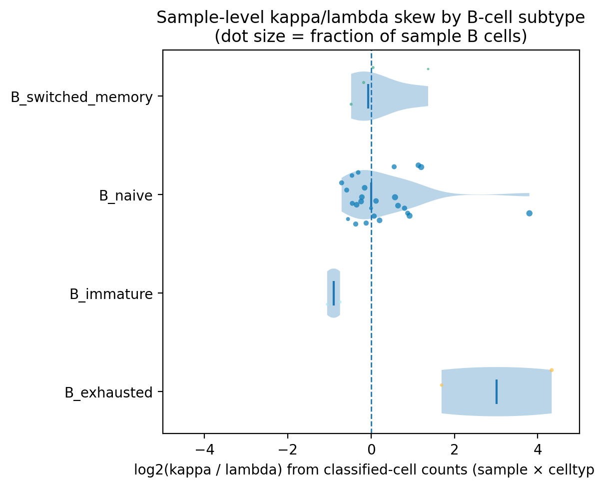
We perform a permutation test to identify cell types enriched for cells with unusually large clone size scores. Cell type labels are randomly shuffled while keeping clone size scores fixed, and the proportion of cells exceeding the reference threshold are recalculated for each permutation. This generates a null distribution against which the observed proportion is compared to determine whether the enrichment of high clone size scores is greater than expected by chance.
We use naive B cells as reference as they are not supposed to be clonal and set a percentile of the reference distribution that we consider to indicate sufficient deviation from polyclonality.
[17]:
res = c2c.permutation_test(
    df_class,
    reference_celltype="B_naive",
    celltype_col=celltype,
    sample_col=sample,
    percentile=0.975,
    n_perms=10000,
    min_samples=2
)
res
[17]:
| celltype | reference_celltype | percentile | threshold | n_samples | n_exceeding | pct_exceeding | p_perm | q_perm | |
|---|---|---|---|---|---|---|---|---|---|
| 0 | B_exhausted | B_naive | 0.975 | 0.486489 | 2 | 1 | 50.0 | 0.129287 | 0.387861 |
| 1 | B_switched_memory | B_naive | 0.975 | 0.486489 | 4 | 0 | 0.0 | 1.000000 | 1.000000 |
| 2 | B_immature | B_naive | 0.975 | 0.486489 | 2 | 0 | 0.0 | 1.000000 | 1.000000 |
Here none of the cell types reach significance due to a relatively small dataset.
[18]:
# define significance
alpha = 0.05
res["significant"] = res["q_perm"] < alpha

# table of significant hits (for figure annotation or reporting)
res_sig = res.loc[res["significant"]].sort_values("q_perm")
res_sig
[18]:
| celltype | reference_celltype | percentile | threshold | n_samples | n_exceeding | pct_exceeding | p_perm | q_perm | significant |
|---|
[19]:
fig, ax = c2c.plot_clone_size_score_violin(
    df_class,
    res=res,
    celltype_col=celltype,
)
plt.show()
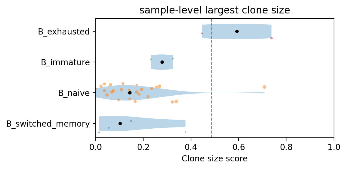
We identify two samples above the threshold defined based on naive B cell distribution. One sample has a putative clonal expansion in exhausted B cells, and the other in naive B cells, which is unexpected.
[20]:
# Add clonality information to adata
adata = c2c.add_df_class_to_adata_obs(
    adata,
    df_class,
    sample_col=sample,
    celltype_col=celltype,
)
[21]:
sc.pl.umap(
    adata,
    color=["clone_size_score", "frac_kappa", celltype],
    frameon=False,
)
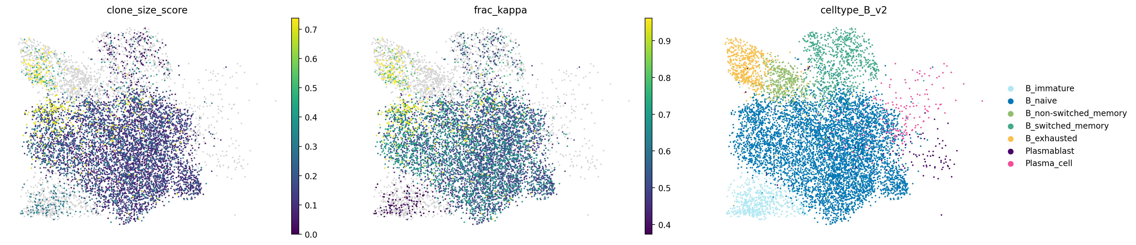
Here the clonality information is defined at the level of pre-annotated cell types. We next look at how to assign single cells to clones independent of prior cell type annotation, which may provide higher resolution and identify clones comprising only a subset of a cell type in a sample.
Assigning single cells to clones
We next select a highly clonal sample/cell type and examine it as single-cell resolution, starting with exhausted B cells.
[22]:
res = c2c.subset_top_bottom_clonal_samples(
    df_clono=df_class,
    adata=adata,
    celltype_col=celltype,
    sample_col=sample,
    frac_celltype="B_exhausted",
    frac_percentile=0.5,
    top_n=1,
    bottom_n=0,
    score_agg="max",
)

print("Celltype frac threshold used:", res["frac_threshold"])
print("Top samples:", res["top_samples"])
print("Bottom samples:", res["bottom_samples"])

adata_sub = res["adata_selected"]
Celltype frac threshold used: 0.17603711790393012
Top samples: ['MH8919330']
Bottom samples: []
We identify highly variable genes after excluding TCR/BCR genes and compute PCA, neighbours and UMAP.
[23]:
# --- define gene families to exclude ---
exclude_regex = (
    r"^TR[ABDG][CDVJ]"   # TCR alpha/beta/delta/gamma (V/C/J)
    r"|^TRAC|^TRBC"     # TCR constant chains
    r"|^IG[HKL][VCJD]" # Ig heavy/kappa/lambda
    r"|^IGH|^IGK|^IGL"  # safety net
)

exclude_mask = adata_sub.var_names.str.contains(
    exclude_regex, regex=True
)

print(f"Excluding {exclude_mask.sum()} TCR/Ig genes from HVG selection")

# --- HVG selection on filtered gene set ---
adata_hvg = adata_sub[:, ~exclude_mask].copy()

sc.pp.highly_variable_genes(adata_hvg)

# --- map HVGs back to full adata_sub ---
hvg = np.zeros(adata_sub.n_vars, dtype=bool)
hvg[~exclude_mask] = adata_hvg.var["highly_variable"].values
adata_sub.var["highly_variable"] = hvg

# --- downstream ---
sc.tl.pca(adata_sub, use_highly_variable=True)
sc.pp.neighbors(adata_sub, use_rep="X_pca")
sc.tl.umap(adata_sub)
Excluding 644 TCR/Ig genes from HVG selection
We assign single cells to clones based on Leiden clusters containing one light/constant chain class above a purity cutoff. Here clones are called if a Leiden cluster is at least 80% pure. If multiple samples are included in the object, Leiden clustering is performed sample-wise as putative clones will be restricted to individuals.
[24]:
c2c.leiden_chain_clones_sampleaware(
    adata_sub,
    class_col="KL_class",
    valid_states=("kappa","lambda"),
    sample_col=sample,
    resolution=1,
    purity_cutoff=0.8,
    key_added="clone_call",
)
[24]:
AnnData object with n_obs × n_vars = 229 × 31279
    obs: 'sample_id', 'n_genes', 'n_genes_by_counts', 'total_counts', 'total_counts_mt', 'pct_counts_mt', 'leiden', 'initial_clustering', 'Resample', 'Collection_Day', 'patient_id', 'Sex', 'Age', 'Ethnicity', 'Swab_result', 'Status', 'Smoker', 'Status_on_day_collection', 'Status_on_day_collection_summary', 'Status_3_days_post_collection', 'Status_7_days_post_collection', 'Days_from_onset', 'Site', 'time_after_LPS', 'Worst_Clinical_Status', 'Outcome', 'filter_rna', 'has_bcr', 'filter_bcr_quality', 'filter_bcr_heavy', 'filter_bcr_light', 'bcr_QC_pass', 'filter_bcr', 'initial_clustering_B', 'leiden_B', 'leiden_B2', 'celltype_B', 'celltype_B_v2', 'clone_id', 'clone_id_by_size', 'isotype', 'lightchain', 'status', 'vdj_status', 'productive', 'umi_counts_heavy', 'umi_counts_light', 'v_call_heavy', 'v_call_light', 'j_call_heavy', 'j_call_light', 'c_call_heavy', 'c_call_light', 'clone_centrality', 'clone_degree', 'clone_id_size', 'mu_freq_heavy', 'mu_freq_light', 'clone_id_size_max_3', 'clone_network_cluster_size_gini', 'clone_network_vertex_size_gini', 'clone_size_gini', 'clone_centrality_gini', 'junction_heavy', 'junction_light', 'junction_aa_heavy', 'junction_aa_light', 'kappa_sum', 'lambda_sum', 'KL_class', 'KL_log_ratio', 'kappa', 'lambda', 'frac_kappa', 'KL_class_log2_ratio_scaled', 'clonality', 'clone_size_score', 'sample_rank_class', 'sample_rank_score', 'sample_frac_B_exhausted', 'clone_call', 'clone_call_id'
    var: 'feature_types', 'highly_variable', 'means', 'dispersions', 'dispersions_norm'
    uns: 'Site_colors', 'Status_on_day_collection_summary_colors', 'bcr_QC_pass_colors', 'celltype_B_colors', 'celltype_B_v2_colors', 'filter_bcr_colors', 'hvg', 'initial_clustering_colors', 'isotype_colors', 'leiden', 'leiden_B_colors', 'leiden_colors', 'neighbors', 'pca', 'rank_genes_groups', 'rna_neighbors', 'umap', 'sample_id_colors', 'clone_call_summary'
    obsm: 'X_bcr', 'X_pca', 'X_pca_harmony', 'X_umap'
    varm: 'PCs'
    obsp: 'bcr_connectivities', 'bcr_distances', 'connectivities', 'distances', 'rna_connectivities', 'rna_distances'
[25]:
sc.pl.umap(adata_sub, color=[sample, celltype, 'KL_class', 'clone_call'], ncols=2, wspace=0.3)
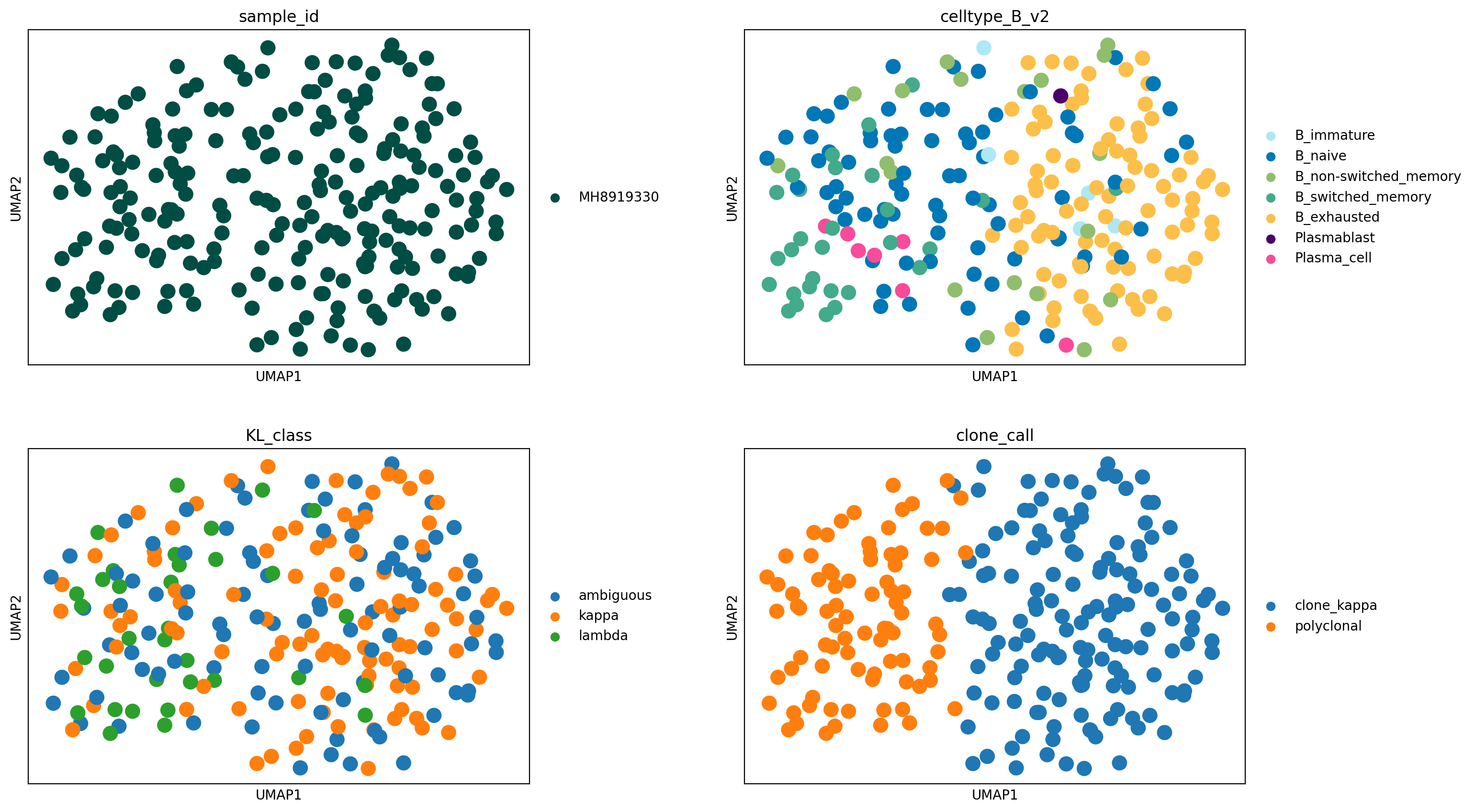
We identify a large expansion of exhausted B cells in this sample, which cell2clone infers to be clonal and kappa light chain-restricted. From KL_class we see how the polyclonal cell population contains a mixture of kappa and lambda B cells, whereas the clonal population contains almost exclusively kappa B cells (in addition to ambiguous cells due to dropouts). Here essentially all exhausted B cells in this sample appear to consist of a single expanded clone.
We next examine BCR sequencing data to confirm the inference.
[26]:
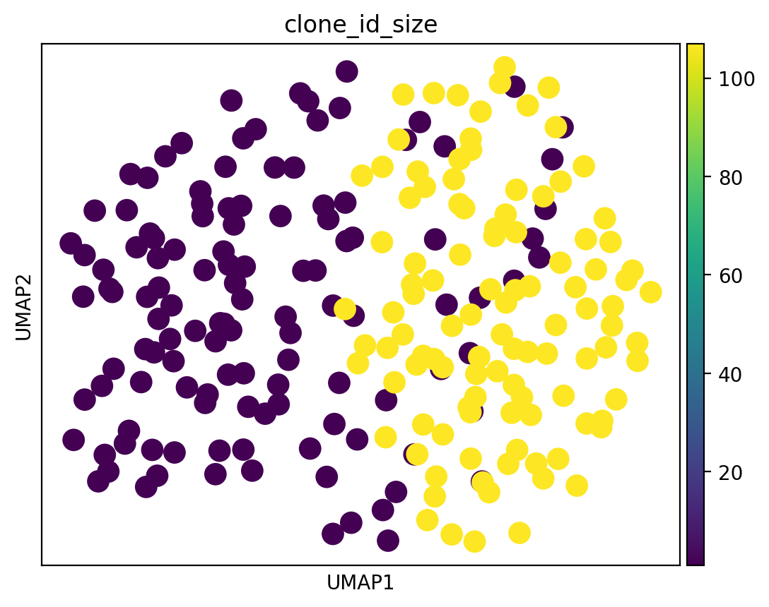
sc.pl.umap(adata_sub, color=['clone_id_size'])
[27]:
# Find the largest clone and plot it on UMAP

# largest clone
largest_clone = (
    adata_sub.obs["clone_id"]
    .astype(str)
    .value_counts()
    .idxmax()
)

largest_n = (
    adata_sub.obs["clone_id"]
    .astype(str)
    .value_counts()
    .max()
)

# annotation for plotting
adata_sub.obs["largest_clone"] = pd.Categorical(
    adata_sub.obs["clone_id"]
    .astype(str)
    .eq(largest_clone)
    .map({True: largest_clone, False: "other"}),
    categories=["other", largest_clone]
)

# UMAP
sc.pl.umap(
    adata_sub,
    color="largest_clone",
    palette=["lightgrey", "darkred"],
    title=f"Largest clone: {largest_clone} (n={largest_n})"
)
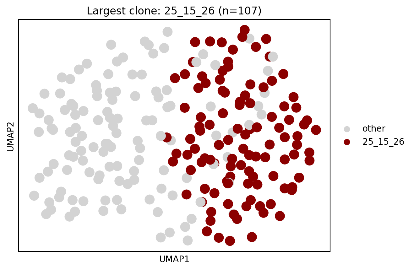
We next check the other sample suggested to contain a clonal expansion based on cell2clone (in naive B cells).
[28]:
res = c2c.subset_top_bottom_clonal_samples(
    df_clono=df_class,
    adata=adata,
    celltype_col=celltype,
    sample_col=sample,
    frac_celltype="B_naive",
    frac_percentile=0,
    top_n=1,
    bottom_n=0,
    score_agg="max",
)

print("Celltype frac threshold used:", res["frac_threshold"])
print("Top samples:", res["top_samples"])
print("Bottom samples:", res["bottom_samples"])

adata_sub = res["adata_selected"]
Celltype frac threshold used: 0.2052401746724891
Top samples: ['BGCV07_CV0094']
Bottom samples: []
[29]:
# --- define gene families to exclude ---
exclude_regex = (
    r"^TR[ABDG][CDVJ]"   # TCR alpha/beta/delta/gamma (V/C/J)
    r"|^TRAC|^TRBC"     # TCR constant chains
    r"|^IG[HKL][VCJD]" # Ig heavy/kappa/lambda
    r"|^IGH|^IGK|^IGL"  # safety net
)

exclude_mask = adata_sub.var_names.str.contains(
    exclude_regex, regex=True
)

print(f"Excluding {exclude_mask.sum()} TCR/Ig genes from HVG selection")

# --- HVG selection on filtered gene set ---
adata_hvg = adata_sub[:, ~exclude_mask].copy()

sc.pp.highly_variable_genes(adata_hvg)

# --- map HVGs back to full adata_sub ---
hvg = np.zeros(adata_sub.n_vars, dtype=bool)
hvg[~exclude_mask] = adata_hvg.var["highly_variable"].values
adata_sub.var["highly_variable"] = hvg

# --- downstream ---
sc.tl.pca(adata_sub, use_highly_variable=True)
sc.pp.neighbors(adata_sub, use_rep="X_pca")
sc.tl.umap(adata_sub)
Excluding 644 TCR/Ig genes from HVG selection
[30]:
c2c.leiden_chain_clones_sampleaware(
    adata_sub,
    class_col="KL_class",
    valid_states=("kappa","lambda"),
    sample_col=sample,
    resolution=1,
    purity_cutoff=0.9,
    key_added="clone_call",
)
[30]:
AnnData object with n_obs × n_vars = 336 × 31279
    obs: 'sample_id', 'n_genes', 'n_genes_by_counts', 'total_counts', 'total_counts_mt', 'pct_counts_mt', 'leiden', 'initial_clustering', 'Resample', 'Collection_Day', 'patient_id', 'Sex', 'Age', 'Ethnicity', 'Swab_result', 'Status', 'Smoker', 'Status_on_day_collection', 'Status_on_day_collection_summary', 'Status_3_days_post_collection', 'Status_7_days_post_collection', 'Days_from_onset', 'Site', 'time_after_LPS', 'Worst_Clinical_Status', 'Outcome', 'filter_rna', 'has_bcr', 'filter_bcr_quality', 'filter_bcr_heavy', 'filter_bcr_light', 'bcr_QC_pass', 'filter_bcr', 'initial_clustering_B', 'leiden_B', 'leiden_B2', 'celltype_B', 'celltype_B_v2', 'clone_id', 'clone_id_by_size', 'isotype', 'lightchain', 'status', 'vdj_status', 'productive', 'umi_counts_heavy', 'umi_counts_light', 'v_call_heavy', 'v_call_light', 'j_call_heavy', 'j_call_light', 'c_call_heavy', 'c_call_light', 'clone_centrality', 'clone_degree', 'clone_id_size', 'mu_freq_heavy', 'mu_freq_light', 'clone_id_size_max_3', 'clone_network_cluster_size_gini', 'clone_network_vertex_size_gini', 'clone_size_gini', 'clone_centrality_gini', 'junction_heavy', 'junction_light', 'junction_aa_heavy', 'junction_aa_light', 'kappa_sum', 'lambda_sum', 'KL_class', 'KL_log_ratio', 'kappa', 'lambda', 'frac_kappa', 'KL_class_log2_ratio_scaled', 'clonality', 'clone_size_score', 'sample_rank_class', 'sample_rank_score', 'sample_frac_B_naive', 'clone_call', 'clone_call_id'
    var: 'feature_types', 'highly_variable', 'means', 'dispersions', 'dispersions_norm'
    uns: 'Site_colors', 'Status_on_day_collection_summary_colors', 'bcr_QC_pass_colors', 'celltype_B_colors', 'celltype_B_v2_colors', 'filter_bcr_colors', 'hvg', 'initial_clustering_colors', 'isotype_colors', 'leiden', 'leiden_B_colors', 'leiden_colors', 'neighbors', 'pca', 'rank_genes_groups', 'rna_neighbors', 'umap', 'sample_id_colors', 'clone_call_summary'
    obsm: 'X_bcr', 'X_pca', 'X_pca_harmony', 'X_umap'
    varm: 'PCs'
    obsp: 'bcr_connectivities', 'bcr_distances', 'connectivities', 'distances', 'rna_connectivities', 'rna_distances'
[31]:
sc.pl.umap(adata_sub, color=[sample, celltype, 'KL_class', 'clone_call'], ncols=2, wspace=0.3)
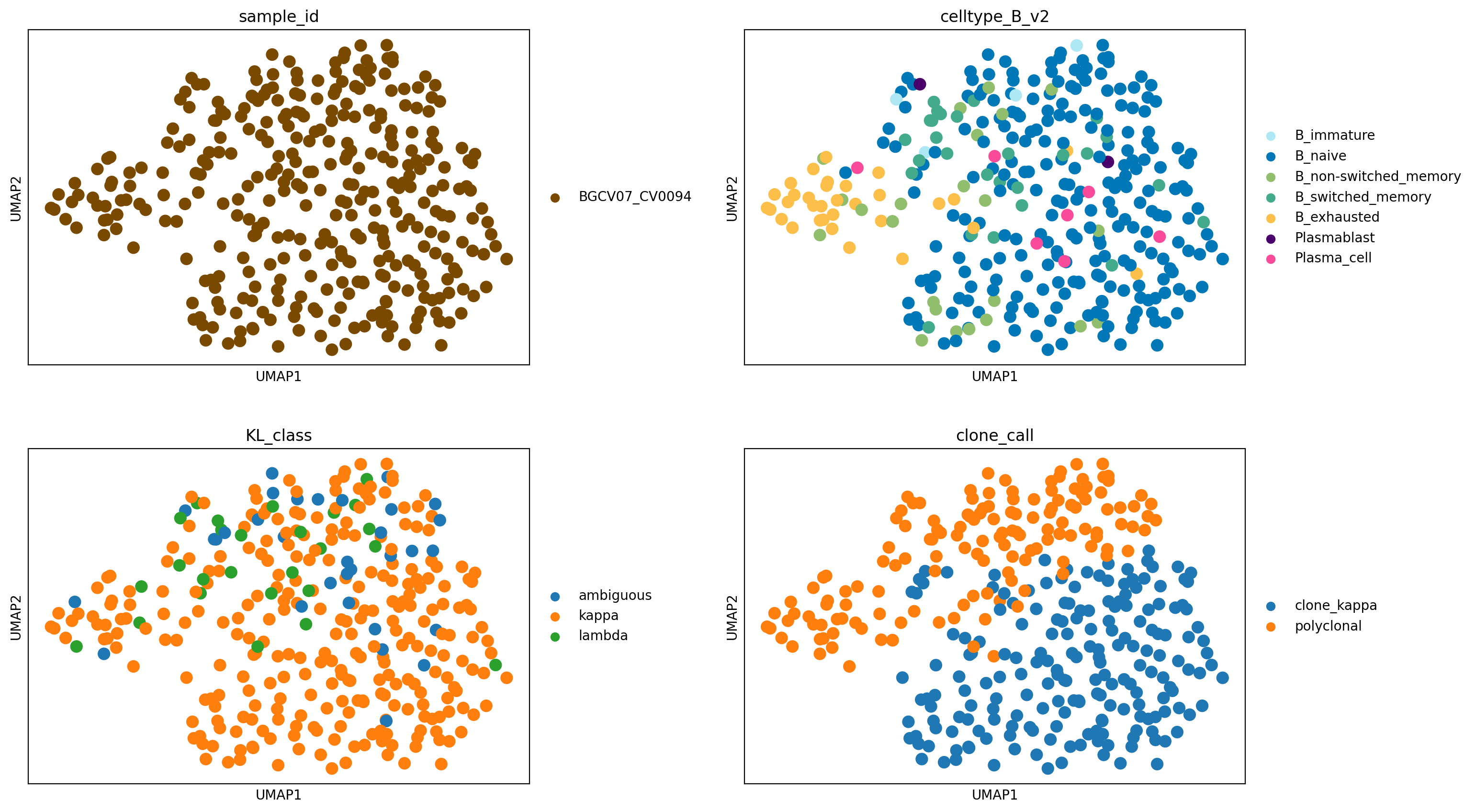
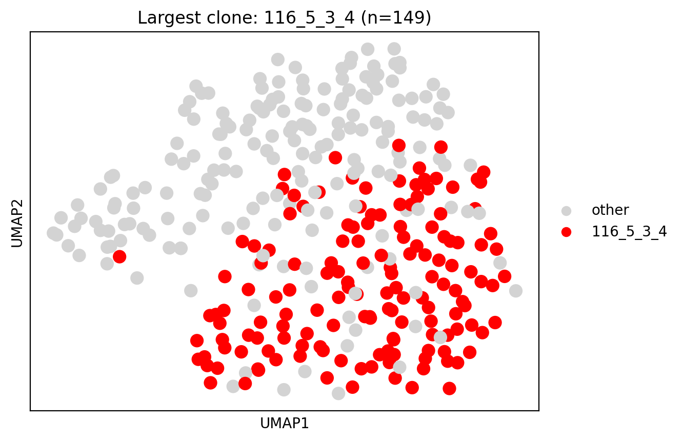
We again identify a large B cell expansion predicted to be clonal and kappa light chain-restricted, in a subset of B cells annotated as B_naive. We again examine BCR sequencing data to confirm the inference.
[32]:
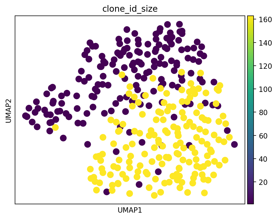
sc.pl.umap(adata_sub, color=['clone_id_size'])
[33]:
# Find the largest clone and plot it on UMAP

# largest clone
largest_clone = (
    adata_sub.obs["clone_id"]
    .astype(str)
    .value_counts()
    .idxmax()
)

largest_n = (
    adata_sub.obs["clone_id"]
    .astype(str)
    .value_counts()
    .max()
)

# annotation for plotting
adata_sub.obs["largest_clone"] = pd.Categorical(
    adata_sub.obs["clone_id"]
    .astype(str)
    .eq(largest_clone)
    .map({True: largest_clone, False: "other"}),
    categories=["other", largest_clone]
)

# UMAP
sc.pl.umap(
    adata_sub,
    color="largest_clone",
    palette=["lightgrey", "red"],
    title=f"Largest clone: {largest_clone} (n={largest_n})"
)
[34]:
adata
[34]:
AnnData object with n_obs × n_vars = 8604 × 31279
    obs: 'sample_id', 'n_genes', 'n_genes_by_counts', 'total_counts', 'total_counts_mt', 'pct_counts_mt', 'leiden', 'initial_clustering', 'Resample', 'Collection_Day', 'patient_id', 'Sex', 'Age', 'Ethnicity', 'Swab_result', 'Status', 'Smoker', 'Status_on_day_collection', 'Status_on_day_collection_summary', 'Status_3_days_post_collection', 'Status_7_days_post_collection', 'Days_from_onset', 'Site', 'time_after_LPS', 'Worst_Clinical_Status', 'Outcome', 'filter_rna', 'has_bcr', 'filter_bcr_quality', 'filter_bcr_heavy', 'filter_bcr_light', 'bcr_QC_pass', 'filter_bcr', 'initial_clustering_B', 'leiden_B', 'leiden_B2', 'celltype_B', 'celltype_B_v2', 'clone_id', 'clone_id_by_size', 'isotype', 'lightchain', 'status', 'vdj_status', 'productive', 'umi_counts_heavy', 'umi_counts_light', 'v_call_heavy', 'v_call_light', 'j_call_heavy', 'j_call_light', 'c_call_heavy', 'c_call_light', 'clone_centrality', 'clone_degree', 'clone_id_size', 'mu_freq_heavy', 'mu_freq_light', 'clone_id_size_max_3', 'clone_network_cluster_size_gini', 'clone_network_vertex_size_gini', 'clone_size_gini', 'clone_centrality_gini', 'junction_heavy', 'junction_light', 'junction_aa_heavy', 'junction_aa_light', 'kappa_sum', 'lambda_sum', 'KL_class', 'KL_log_ratio', 'kappa', 'lambda', 'frac_kappa', 'KL_class_log2_ratio_scaled', 'clonality', 'clone_size_score'
    var: 'feature_types', 'highly_variable', 'means', 'dispersions', 'dispersions_norm'
    uns: 'Site_colors', 'Status_on_day_collection_summary_colors', 'bcr_QC_pass_colors', 'celltype_B_colors', 'celltype_B_v2_colors', 'filter_bcr_colors', 'hvg', 'initial_clustering_colors', 'isotype_colors', 'leiden', 'leiden_B_colors', 'leiden_colors', 'neighbors', 'pca', 'rank_genes_groups', 'rna_neighbors', 'umap', 'sample_id_colors'
    obsm: 'X_bcr', 'X_pca', 'X_pca_harmony', 'X_umap'
    obsp: 'bcr_connectivities', 'bcr_distances', 'connectivities', 'distances', 'rna_connectivities', 'rna_distances'
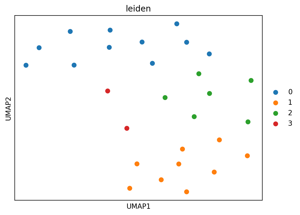
Cluster samples based on clonality across cell types
Finally, we identify groups of samples with clonal expansions in same cell types. This analysis is more informative with larger datasets but the approch is shown here as an example.
[35]:
# Make data frame of sample x celltype-specific clonality/clone size score

def wide_multi(df, value_cols):
    wide = (
        df
        .pivot_table(
            index=sample,
            columns=celltype,
            values=value_cols,
            aggfunc="first"
        )
    )

    # flatten multiindex columns
    wide.columns = [
        f"{ct}_{metric}"
        for metric, ct in wide.columns
    ]

    return wide


df_class_wide = wide_multi(df_class, ["clonality", "clone_size_score"])
[36]:
df_class_wide
[36]:
| B_immature_clonality | B_naive_clonality | B_switched_memory_clonality | B_exhausted_clonality | B_immature_clone_size_score | B_naive_clone_size_score | B_switched_memory_clone_size_score | B_exhausted_clone_size_score | |
|---|---|---|---|---|---|---|---|---|
| sample_id | ||||||||
| AP3 | NaN | 0.878756 | NaN | 1.691878 | NaN | 0.255994 | NaN | 0.446154 |
| AP9 | NaN | 0.553235 | NaN | NaN | NaN | 0.172751 | NaN | NaN |
| BGCV01_CV0025 | NaN | 0.119299 | NaN | NaN | NaN | 0.036765 | NaN | NaN |
| BGCV02_CV0052 | NaN | 0.803771 | NaN | NaN | NaN | 0.235871 | NaN | NaN |
| BGCV06_CV0037 | NaN | 0.575064 | NaN | NaN | NaN | 0.172175 | NaN | NaN |
| BGCV06_CV0234 | NaN | 0.204084 | NaN | NaN | NaN | 0.062630 | NaN | NaN |
| BGCV07_CV0094 | NaN | 3.800402 | NaN | NaN | NaN | 0.708641 | NaN | NaN |
| BGCV07_CV0134 | NaN | 1.135484 | NaN | NaN | NaN | 0.321754 | NaN | NaN |
| BGCV07_CV0137 | NaN | 0.924538 | NaN | NaN | NaN | 0.268083 | NaN | NaN |
| BGCV11_CV0257 | NaN | 1.203777 | NaN | NaN | NaN | 0.338388 | NaN | NaN |
| MH8919330 | NaN | 0.000000 | NaN | 4.335733 | NaN | 0.000000 | NaN | 0.738166 |
| MH8919331 | NaN | 0.457500 | NaN | NaN | NaN | 0.142905 | NaN | NaN |
| MH9143270 | NaN | 0.073748 | NaN | NaN | NaN | 0.022773 | NaN | NaN |
| MH9143275 | NaN | 0.219991 | 0.478047 | NaN | NaN | 0.068555 | 0.149321 | NaN |
| MH9143322 | NaN | 0.706672 | NaN | NaN | NaN | 0.220211 | NaN | NaN |
| MH9143323 | NaN | 0.584640 | NaN | NaN | NaN | 0.182509 | NaN | NaN |
| MH9143324 | NaN | 0.554374 | NaN | NaN | NaN | 0.166253 | NaN | NaN |
| MH9143327 | NaN | 0.308122 | NaN | NaN | NaN | 0.096154 | NaN | NaN |
| MH9143371 | NaN | 0.346596 | NaN | NaN | NaN | 0.108205 | NaN | NaN |
| MH9143423 | 0.744221 | 0.450727 | 0.176878 | NaN | 0.231731 | 0.140788 | 0.055070 | NaN |
| MH9143424 | 1.053549 | 0.238939 | 1.369950 | NaN | 0.324598 | 0.074486 | 0.377289 | NaN |
| MH9179821 | NaN | 0.153794 | NaN | NaN | NaN | 0.047857 | NaN | NaN |
| MH9179823 | NaN | 0.367829 | NaN | NaN | NaN | 0.114854 | NaN | NaN |
| MH9179824 | NaN | 0.117074 | 0.048022 | NaN | NaN | 0.036395 | 0.014845 | NaN |
| MH9179825 | NaN | 0.647023 | NaN | NaN | NaN | 0.192575 | NaN | NaN |
[37]:
## Create anndata based on clone size score matrix

# 1. Select clone_size_score columns

df_class_wide['sample'] = df_class_wide.index

clone_cols = [c for c in df_class_wide.columns if c.endswith("_clone_size_score")]

# 2. Build sample × celltype matrix
X = (
    df_class_wide[["sample"] + clone_cols]
    .groupby("sample")
    .mean()              # in case sample appears multiple times
)

# 3. Replace NaNs (absence of that celltype in sample at sufficient numbers → 0 clonality)
X = X.fillna(0)

# 4. Create AnnData
adata_clone = sc.AnnData(X)
adata_clone.obs_names = X.index
adata_clone.var_names = X.columns
[38]:
# 5. Highly variable features
sc.pp.highly_variable_genes(adata_clone)

# 6. PCA
sc.tl.pca(adata_clone, svd_solver="arpack")

# 7. Neighbours
sc.pp.neighbors(adata_clone, n_neighbors=15, n_pcs=20) # increase neigbour count when using with more samples

# 8. UMAP
sc.tl.umap(adata_clone)

# 9. Leiden clustering
sc.tl.leiden(adata_clone, resolution=1)

# 10. Plot
sc.pl.umap(adata_clone, color=["leiden"], size=200)
[39]:
sc.pl.umap(adata_clone, color=adata_clone.var_names, size=200)
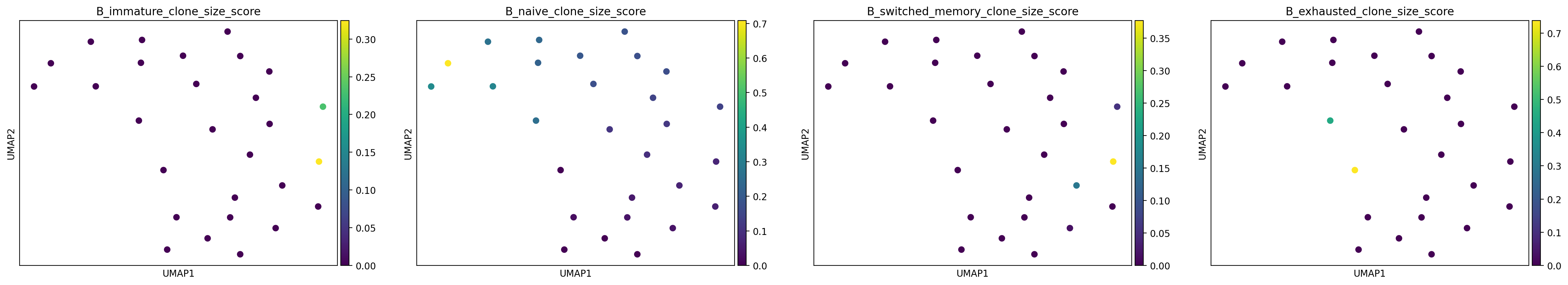
Using this approach, we can visualise cell type-specific clonality across donors and identify groups of donors where certain cell types are clonally expanded.